Observation Models¶

Two observation models are provided, both of which related disease incidence in the simulation model to count data, but differ in how they treat the denominator.

Observations from the entire population¶

The PopnCounts class provides a generic observation model for relating disease incidence to count data where the denominator is assumed to be the population size \(N\) (i.e., the denominator is assumed constant and is either not known or is known to be the population size \(N\)).

This observation model assumes that the relationship between observed case counts \(y_t\) and disease incidence in particle \(x_t\) follow a negative binomial distribution with mean \(\mathbb{E}[y_t]\) and dispersion parameter \(k\).

\[\begin{split}\mathcal{L}(y_t \mid x_t) &\sim NB(\mathbb{E}[y_t], k)\end{split}\]\[\begin{split}\mathbb{E}[y_t] &= (1 - p_\mathrm{inf}) \cdot bg_\mathrm{obs} + p_\mathrm{inf} \cdot p_\mathrm{obs} \cdot N\end{split}\]\[\begin{split}\operatorname{Var}[y_t] &= \mathbb{E}[y_t] + \frac{\left(\mathbb{E}[y_t]\right)^2}{k}\end{split}\]

The observation model parameters comprise:

The background observation rate \(bg_\mathrm{obs}\);
The probability of observing an infected individual \(p_\mathrm{obs}\); and
The dispersion parameter \(k\), which controls the relationship between the mean \((\mathbb{E}[y_t])\) and the variance; as \(k \to \infty\) the distribution approaches the Poisson, as \(k \to 0\) the distribution becomes more and more over-dispersed with respect to the Poisson.

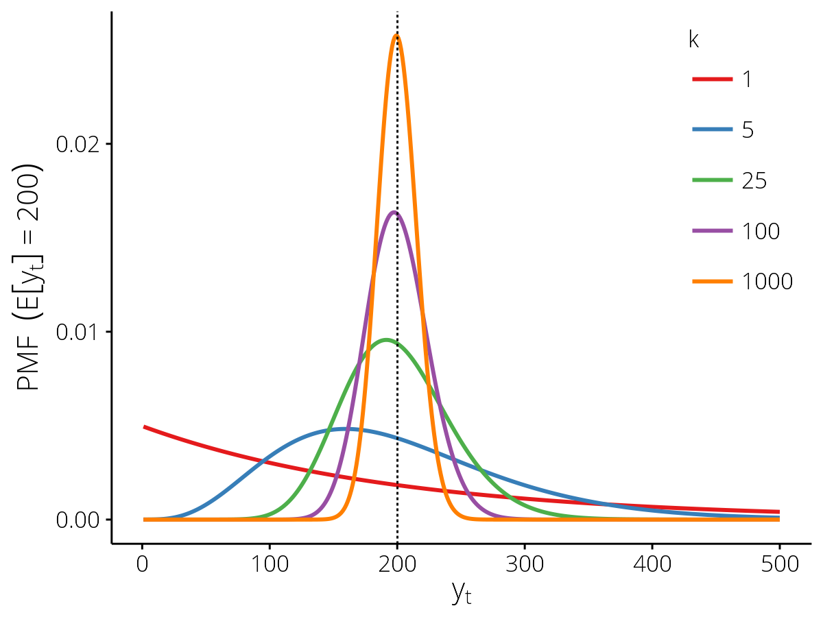
Probability mass functions for the PopnCounts observation model with different values of the dispersion parameter \(k\), for the expected value \(\mathbb{E}[y_t] = 200\) (vertical dashed line).

class epifx.obs.PopnCounts(obs_unit, obs_period, pr_obs_ix=None)¶

Generic observation model for relating disease incidence to count data where the denominator is assumed or known to be the population size.

Parameters:	obs_unit – A descriptive name for the data. obs_period – The observation period (in days). pr_obs_ix – The index of the model parameter that defines the observation probability (\(p_\mathrm{obs}\)). By default, the value in the parameters dictionary is used.

expect(params, op, period, pr_inf, prev, curr)¶: Calculate the expected observation value \(\mathbb{E}[y_t]\) for every particle \(x_t\).

log_llhd(params, op, obs, pr_indiv, curr, hist)¶

Calculate the log-likelihood \(\mathcal{l}(y_t \mid x_t)\) for the observation \(y_t\) (obs) and every particle \(x_t\).

If it is known (or suspected) that the observed value will increase in the future — when obs['incomplete'] == True — then the log-likehood \(\mathcal{l}(y > y_t \mid x_t)\) is calculated instead (i.e., the log of the survival function).

If an upper bound to this increase is also known (or estimated) — when obs['upper_bound'] is defined — then the log-likelihood \(\mathcal{l}(y_u \ge y > y_t \mid x_t)\) is calculated instead.

define_params(params, bg_obs, pr_obs, disp)¶

Add observation model parameters to the simulation parameters.

Parameters:	bg_obs – The background signal in the data (\(bg_\mathrm{obs}\)). pr_obs – The probability of observing an infected individual (\(p_\mathrm{obs}\)). disp – The dispersion parameter (\(k\)).

from_file(filename, year=None, date_col=u'to', value_col=u'count')¶

Load count data from a space-delimited text file with column headers defined in the first line.

Parameters:	filename – The file to read. year – Only returns observations for a specific year. The default behaviour is to return all recorded observations. date_col – The name of the observation date column. value_col – The name of the observation value column.
Returns:	A list of observations, ordered as per the original file.

Observations from population samples¶

The SampleCounts class provides a generic observation model for relating disease incidence to count data where the denominator is reported and may vary (e.g., weekly counts of all patients and the number that presented with influenza-like illness), and where the background signal is not a fixed value but rather a fixed proportion.

For this observation model, each observed value \((y_t)\) is the fraction of all patients \((N_t)\) that were identified as cases \((c_t)\). This observation model assumes that the relationship between the observed fraction \(y_t\), the denominator \(N_t\), and disease incidence in particle \(x_t\) follows a Beta-binomial distribution with probability of success \(\mathbb{E}[y_t]\) and dispersion parameter \(k\).

\[\begin{split}\mathcal{L}(c_t \mid N_t, x_t) &\sim \operatorname{BetaBin}(N_t, \mathbb{E}[y_t], k)\end{split}\]\[\begin{split}\mathbb{E}[c_t] &= N_t \cdot \mathbb{E}[y_t]\end{split}\]\[\begin{split}\operatorname{Var}[c_t] &= N_t \cdot p \cdot (1 - p) \cdot \left[ 1 + \frac{N_t - 1}{k + 1} \right]\end{split}\]\[\begin{split}\mathbb{E}[y_t] &= bg_\mathrm{obs} + p_\mathrm{inf} \cdot \kappa_\mathrm{obs}\end{split}\]\[\begin{split}y_t &= \frac{c_t}{N_t}\end{split}\]

The shape parameters \(\alpha\) and \(\beta\) satisfy:

\[\begin{split}p &= \mathbb{E}[y_t] = \frac{\alpha}{\alpha + \beta}\end{split}\]\[\begin{split}k &= \alpha + \beta\end{split}\]\[\begin{split}\implies \alpha &= p \cdot k\end{split}\]\[\begin{split}\implies \beta &= (1 - p) \cdot k\end{split}\]

The observation model parameters comprise:

The background case fraction \(bg_\mathrm{obs}\);
The slope \(\kappa_\mathrm{obs}\) of the relationship between disease incidence and the proportion of cases; and
The dispersion parameter \(k\), which controls the relationship between the mean \((\mathbb{E}[y_t])\) and the variance; as \(k \to \infty\) the distribution approaches the binomial, as \(k \to 0\) the distribution becomes more and more over-dispersed with respect to the binomial.

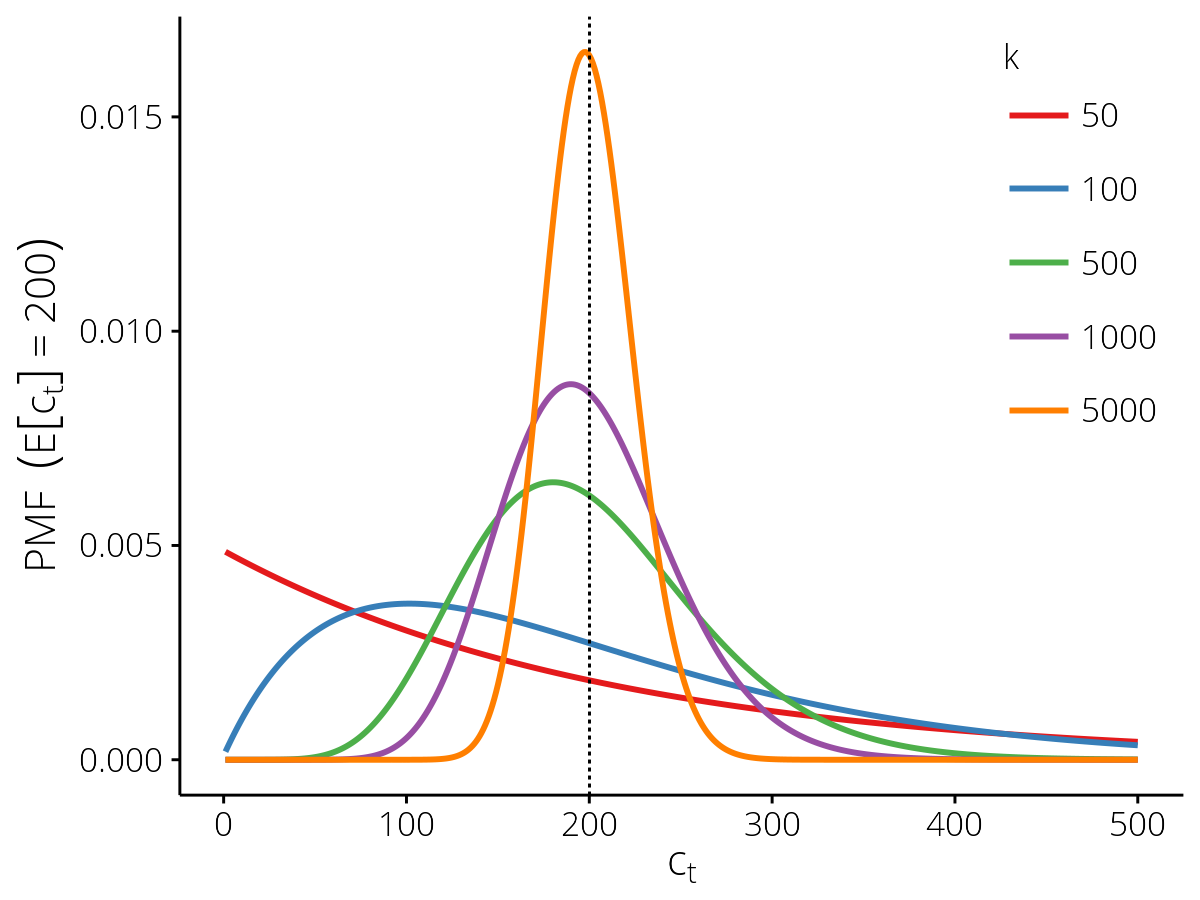
Probability density functions for the SampleCounts observation model.

Probability mass functions for the SampleCounts observation model with different values of the dispersion parameter \(k\), for the expected value \(\mathbb{E}[c_t] = 200\) (vertical dashed line) where \(\mathbb{E}[y_t] = 0.02\) and \(N_t = 10,\!000\).

class epifx.obs.SampleCounts(obs_unit, obs_period, k_obs_ix=None)¶

Generic observation model for relating disease incidence to count data where the denominator is reported.

Parameters:	obs_unit – A descriptive name for the data. obs_period – The observation period (in days). k_obs_ix – The index of the model parameter that defines the disease-related increase in observation rate (\(\kappa_\mathrm{obs}\)). By default, the value in the parameters dictionary is used.

expect(params, op, period, pr_inf, prev, curr)¶: Calculate the expected observation value \(\mathbb{E}[y_t]\) for every particle \(x_t\).

log_llhd(params, op, obs, pr_indiv, curr, hist)¶

Calculate the log-likelihood \(\mathcal{l}(y_t \mid x_t)\) for the observation \(y_t\) (obs) and every particle \(x_t\).

If it is known (or suspected) that the observed value will increase in the future — when obs['incomplete'] == True — then the log-likehood \(\mathcal{l}(y > y_t \mid x_t)\) is calculated instead (i.e., the log of the survival function).

If an upper bound to this increase is also known (or estimated) — when obs['upper_bound'] is defined — then the log-likelihood \(\mathcal{l}(y_u \ge y > y_t \mid x_t)\) is calculated instead.

define_params(params, bg_obs, k_obs, disp)¶

Add observation model parameters to the simulation parameters.

Parameters:	bg_obs – The background signal in the data (\(bg_\mathrm{obs}\)). k_obs – The increase in observation rate due to infected individuals (\(\kappa_\mathrm{obs}\)). disp – The dispersion parameter (\(k\)).

from_file(filename, year=None, date_col=u'to', value_col=u'cases', denom_col=u'patients')¶

Load count data from a space-delimited text file with column headers defined in the first line.

Note that returned observation values represent the fraction of patients that were counted as cases, not the absolute number of cases. The number of cases and the number of patients are recorded under the 'numerator' and 'denominator' keys, respectively.

Parameters:	filename – The file to read. year – Only returns observations for a specific year. The default behaviour is to return all recorded observations. date_col – The name of the observation date column. value_col – The name of the observation value column (reported as absolute values, not fractions). denom_col – The name of the observation denominator column.
Returns:	A list of observations, ordered as per the original file.
Raises:	ValueError – If a denominator or value is negative, or if the value exceeds the denominator.

Reading observations from disk¶

The from_file() methods provided by the observation models listed above use read_table() to read specific columns from data files. This function is intended to be a flexible wrapper around numpy.loadtxt, and should be sufficient for reading almost any whitespace-delimited data file with named columns.

epifx.obs.read_table(filename, columns, date_fmt=None, comment=u'#')¶

Load data from a space-delimited ASCII text file with column headers defined in the first non-comment line.

Parameters:	filename – The file to read. columns – The columns to read, represented as a list of `(name, type)` tuples; `type` should either be a built-in NumPy scalar type, or `datetime.date` or `datetime.datetime` (in which case string values will be automatically converted to `datetime.datetime` objects by `datetime_conv()`). date_fmt – A format string for parsing date columns; see `datetime_conv()` for details and the default format string. comment – Prefix string(s) that identify comment lines; either a single Unicode string or a tuple of Unicode strings.
Returns:	A NumPy structured array.
Raises:	ValueError – If the data file contains non-ASCII text (i.e., bytes greater than 127), because `numpy.loadtxt` cannot process non-ASCII data (e.g., see NumPy issues #3184, #4543, #4600, #4939).
Example:

The code below demonstrates how to read observations from a file that includes columns for the year, the observation date, the observed value, and free-text metadata (up to 20 characters in length).

import datetime
import numpy as np
import epifx.obs
columns = [('year', np.int32), ('date', datetime.datetime),
           ('count', np.int32), ('metadata', 'S20')]
df = epifx.obs.read_table('my-data-file.ssv', columns,
                          date_fmt='%Y-%m-%d')

epifx.obs.datetime_conv(text, fmt=u'%Y-%m-%d', encoding=u'utf-8')¶

Convert date strings to datetime.datetime instances. This is a convenience function intended for use with, e.g., numpy.loadtxt.

Parameters:	text – A string (bytes or Unicode) containing a date or date-time. fmt – A format string that defines the textual representation. See the Python `strptime` documentation for details. encoding – The byte string encoding (default is UTF-8).